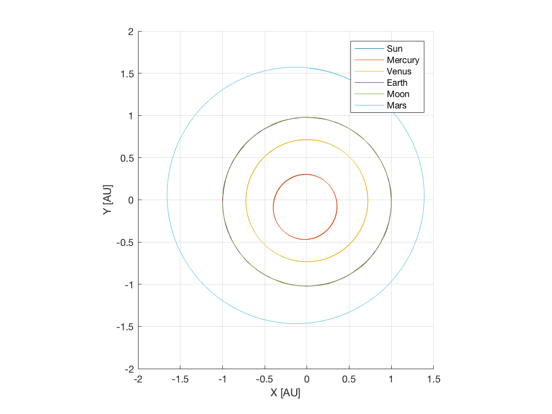
Inner Solar System Propagation

This tutorial describes how the orbit of the inner Solar system bodies can be propagated using the MATLAB Interface, similar to the example Inner Solar System Propagation written in C++. The code for this example can be found at:

tudatBundle/matlabInterface/Examples/Seamless/innerSolarSystem.m

The first step is to include the source code of the MATLAB Interface into MATLAB’s path in the current session so that all the classes needed to set up the simulation can be accessed. This is done by writing:

tudat.load();

Now, we create a Simulation object and specify the initial and final epochs and the global frame orientation:

simulation = Simulation();
simulation.initialEpoch = 1e7;
simulation.finalEpoch = simulation.initialEpoch + convert.toSI(2,'y');
simulation.spice.preloadEphemeris = false;

Note that the function toSI from the convert package has been used to convert 2 years to seconds. In this case, we disable preloading ephemeris of the celestial bodies from Spice, as this is precisely what we are going to propagate.

Next, we create the bodies. There exist predefined objects for celestial bodies (namely the Sun, the Moon and the eight planets), so these objects can be added directly without the need to specify their properties:

simulation.addBodies(Sun,Mercury,Venus,Earth,Moon,Mars);

Now we need to specify the accelerations acting on each body. The accelerations acting on each body are the point-mass gravitational attractions caused by the other bodies. We can define all the accelerations by writing a nested for-loop:

bodyNames = fieldnames(simulation.bodies);
for i = 1:length(bodyNames)
    for j = 1:length(bodyNames)
        if i ~= j
            accelerations.(bodyNames{i}).(bodyNames{j}) = {PointMassGravity()};
        end
    end
end

Note that the names of the bodies have been retrieved from fieldnames(simulation.bodies).

Then, we create the settings for the propagation. We are going to propagate the translational state of the celestial bodies. Thus, we use a TranslationalPropagator:

propagator = TranslationalPropagator();
propagator.bodiesToPropagate = bodyNames;
propagator.centralBodies = repmat({'SSB'},size(bodyNames));
propagator.accelerations = accelerations;
simulation.propagators = {propagator};

In this case, we use an hypothetical central body named SSB (Solar system barycentre) for all the celestial bodies. The built-in function repmat is used to create a cell array containing 'SSB' repeated six times in this case.

Finally, we define the integrator settings, in this case we use a Runge-Kutta 4 integrator with a fixed step-size of one hour:

simulation.integrator.type = Integrators.rungeKutta4;
simulation.integrator.stepSize = 3600;

All the settings needed to run the simulation have been defined. Thus, we can write:

simulation.run();

This method creates a temporary input file and calls the json_interface application, generating a temporary output file containing the state of the satellite for each integration step. Then, it loads these results into the struct results of the simulation object. Finally, all the temporary files are deleted.

After running the simulation, if no specific results have been requested, we can obtain the numerical solution of the equations of motion from simulation.results.numericalSolution. This is a matrix containing in each row the results of an integration step. The first column contains the epochs, while the columns 2 to 7 contain the associated Cartesian states of the first propagated body (the Sun), columns 8 to 13 the Cartesian states of the second propagated body (Mercury), and so on. We can retrieve the positions for each body and save them in the struct r by writing:

for i = 1:length(bodyNames)
    fromIndex = 2 + (i-1)*6;
    toIndex = fromIndex + 2;
    r.(bodyNames{i}) = convert.fromSI(simulation.results.numericalSolution(:,fromIndex:toIndex),'AU');
end

Note the use of the function fromSI of the convert package, which in this case converts metres to astronomical units.

Finally, we generate a plot showing the positions of the celestial bodies during the propagation period of two years, which yields the orbits of the planets:

figure;
hold on;
for i = 1:length(bodyNames)
    bodyPosition = r.(bodyNames{i});
    plot3(bodyPosition(:,1),bodyPosition(:,2),bodyPosition(:,3));
end
legend(bodyNames{:});
axis([-2 2 -2 2 -0.1 0.1]);
axis equal;
grid on;
xlabel('X [AU]');
ylabel('Y [AU]');
zlabel('Z [AU]');
hold off;