Perturbed Earth-orbiting Satellite

This tutorial describes how to propagate the orbit of a perturbed satellite about Earth using the MATLAB Interface, similar to the example Perturbed Earth-orbiting Satellite written in C++. The code for this example can be found at:

tudatBundle/matlabInterface/Examples/Seamless/singlePerturbedSatellite.m

The first step is to include the source code of the MATLAB Interface into MATLAB’s path in the current session so that all the classes needed to set up the simulation can be accessed. This is done by writing:

tudat.load();

Now, we create a Simulation object and specify the initial and final epochs and the global frame orientation:

simulation = Simulation();
simulation.initialEpoch = 0;
simulation.finalEpoch = convert.toSI(1,'d');
simulation.globalFrameOrientation = 'J2000';

Note that the function toSI from the convert package has been used to convert 1 day to seconds. In this case, the global frame origin is not specified because the default value (SSB, Solar system barycentre) is to be used. However, for the global frame orientation the value of J2000 is specified instead of the default ECLIPJ2000.

Next, we create the bodies. In this case, the only non-celestial body is asterix:

asterix = Body('asterix');
asterix.initialState.semiMajorAxis = 7500e3;
asterix.initialState.eccentricity = 0.1;
asterix.initialState.inclination = deg2rad(85.3);
asterix.initialState.argumentOfPeriapsis = deg2rad(235.7);
asterix.initialState.longitudeOfAscendingNode = deg2rad(23.4);
asterix.initialState.trueAnomaly = deg2rad(139.87);
asterix.mass = 400;
asterix.referenceArea = 4;
asterix.dragCoefficient = 1.2;
asterix.radiationPressureCoefficient = 1.2;
asterix.radiationPressure.Sun.occultingBodies = {Earth};

Now, we add the bodies to the simulation by calling the method addBodies of the simulation object. There exist predefined objects for celestial bodies (namely the Sun, the Moon and the eight planets), so these objects can be added directly without the need to specify their properties:

simulation.addBodies(Sun,Earth,Moon,Mars,Venus,asterix);

Now we need to specify the accelerations acting on asterix:

accelerationsOnAsterix.Earth = {SphericalHarmonicGravity(5,5), AerodynamicAcceleration()};
accelerationsOnAsterix.Sun = {PointMassGravity(), RadiationPressureAcceleration()};
accelerationsOnAsterix.Moon = {PointMassGravity()};
accelerationsOnAsterix.Mars = {PointMassGravity()};
accelerationsOnAsterix.Venus = {PointMassGravity()};

Then, we create the settings for the propagation. We are going to propagate the translational state of the body asterix about Earth. Thus, we use a TranslationalPropagator:

propagator = TranslationalPropagator();
propagator.bodiesToPropagate = {asterix};
propagator.centralBodies = {Earth};
propagator.accelerations.asterix = accelerationsOnAsterix;
simulation.propagators = {propagator};

Then, we define the integrator settings, in this case we use a Runge-Kutta 4 integrator with a fixed step-size of 10 seconds:

simulation.integrator.type = Integrators.rungeKutta4;
simulation.integrator.stepSize = 10;

Finally, we specify the results to be saved:

simulation.addResultsToSave('t','independent');
simulation.addResultsToSave('h','asterix.altitude-Earth');

The first variable, named t, represents the independent variable, i.e. the epoch (seconds since J2000). The second variable, named h, represents the altitude of asterix w.r.t. Earth.

All the settings needed to run the simulation have been defined. Thus, we can write:

simulation.run();

This method creates a temporary input file and calls the json_interface application, generating a temporary output file containing the values of the variables that were requested to be saved. Then, it loads these results into the struct results of the simulation object. Finally, all the temporary files are deleted.

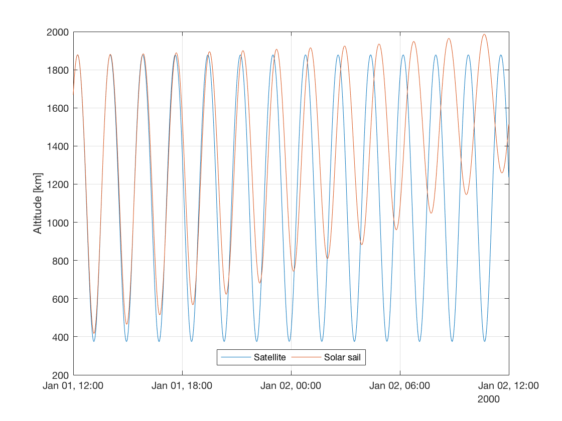
After running the simulation, we can obtain the requested results from simulation.results.t and simulation.results.h, which are column vectors containing the values of these variables at each integration step. We can use the results to generate a plot of the altitude of asterix:

figure;
plot(convert.epochToDate(simulation.results.t),simulation.results.h/1e3);
grid on;
ylabel('Altitude [km]');

Note the use of the epochToDate function of the convert package, which converts seconds since J2000 to a datetime object.

Then, we can run another propagation just by modifying a few parameters. For instance, we can propagate the orbit of a satellite with a larger area and smaller mass, similar to a solar sail. We can do this by writing:

asterix.mass = 4;
asterix.referenceArea = 40;
simulation.run();

Since the class Body derives from handle, whose behaviour is similar to that of a shared pointer, when we modify the body asterix, the property simulation.bodies.asterix is updated automatically. Then, we can run the simulation again (with the updated properties) and use the new results to add a curve to the current plot:

hold on;
plot(convert.epochToDate(simulation.results.t),simulation.results.h/1e3);
hold off;
legend('Satellite','Solar sail','Location','South','Orientation','Horizontal');