Thrust force along velocity vector

This tutorial describes how to propagate the orbit of a perturbed satellite about Earth which has a thrust force directed along the velocity vector using the MATLAB Interface, similar to the example Use of Thrust: Thrust Force Along Velocity Vector written in C++. The code for this example can be found at:

tudatBundle/matlabInterface/Examples/Seamless/thrustAlongVelocityVector.m

The first step is to include the source code of the MATLAB Interface into MATLAB’s path in the current session so that all the classes needed to set up the simulation can be accessed. This is done by writing:

tudat.load();

Now, we create a Simulation object specifying the initial and final epochs (0 and 14 days after J2000):

simulation = Simulation(0,convert.toSI(14,'d'));
simulation.spice.preloadEphemeris = false;

Note that the function toSI from the convert package has been used to convert 14 days to seconds. We disable preloading of the ephemeris for celestial bodies from Spice.

Next, we create the bodies. In this case, the only non-celestial body is vehicle:

vehicle = Body('vehicle');
vehicle.initialState.x = 8e6;
vehicle.initialState.vy = 7500;
vehicle.mass = 5000;

Note that the four components of the cartesian state that have not been specified are assumed to be zero.

Now, we add the bodies to the simulation by calling the method addBodies of the simulation object. There exist predefined objects for celestial bodies (namely the Sun, the Moon and the eight planets), so these objects can be added directly without the need to specify their properties:

simulation.addBodies(Sun,Earth,Moon,vehicle);

Now we need to specify the accelerations acting on vehicle:

accelerationsOnVehicle.Earth = {PointMassGravity()};
accelerationsOnVehicle.Sun = {PointMassGravity()};
accelerationsOnVehicle.Moon = {PointMassGravity()};

In this case, there is another acceleration acting on vehicle: that caused by thrust. Since no objects have been defined for the engines causing the acceleration, we say that thrust is an “acceleration acting on vehicle caused by vehicle”, and thus we will assign it to accelerationsOnVehicle.vehicle. To create the thrust acceleration, we need to provide its direction and magnitude settings:

thrust = Thrust();
thrust.direction.type = ThrustDirections.colinearWithStateSegment;
thrust.direction.relativeBody = Earth;
thrust.direction.colinearWithVelocity = true;
thrust.direction.towardsRelativeBody = false;
thrust.magnitude = ConstantThrustMagnitude();
thrust.magnitude.constantMagnitude = 25;
thrust.magnitude.specificImpulse = 5000;
accelerationsOnVehicle.vehicle = {thrust};

Then, we create the settings for the propagation. We are going to propagate the translational state of the body vehicle about Earth, and also its mass (since propellant is being used to generate thrust, the mass of the body vehicle will change). Thus, we create first a TranslationalPropagator:

translationalPropagator = TranslationalPropagator();
translationalPropagator.bodiesToPropagate = {vehicle};
translationalPropagator.centralBodies = {Earth};
translationalPropagator.accelerations.vehicle = accelerationsOnVehicle;

and then a MassPropagator:

massPropagator = MassPropagator();
massPropagator.bodiesToPropagate = {vehicle};
massPropagator.massRateModels.vehicle = {FromThrustMassRateModel()};

In this case, instead of defining the acceleration models, we have to define the mass-rate models. By using the class FromThrustMassRateModel, the rate of change of the mass of the vehicle is determined from the provided thrust settings for that body.

Once we have created the two propagators, we have to add them to the simulation object:

simulation.propagators = {translationalPropagator, massPropagator};

Then, we define the integrator settings, in this case we use a Runge-Kutta 4 integrator with a fixed step-size of 30 seconds:

simulation.integrator.type = Integrators.rungeKutta4;
simulation.integrator.stepSize = 30;

All the settings needed to run the simulation have been defined. Thus, we can write:

simulation.run();
epochsOn = simulation.results.numericalSolution(:,1);
statesOn = simulation.results.numericalSolution(:,2:7);
masses = simulation.results.numericalSolution(:,8);

Note that we save the values of the epoch, the state and the mass at each integration state to the variables epochsOn, statesOn and masses. Then, we run the simulation again with thrust turned off (by setting its magnitude to zero) and store the results to the variables epochsOff and statesOff (in this case the mass is constant):

thrust.magnitude.constantMagnitude = 0;
simulation.run();
epochsOff = simulation.results.numericalSolution(:,1);
statesOff = simulation.results.numericalSolution(:,2:7);

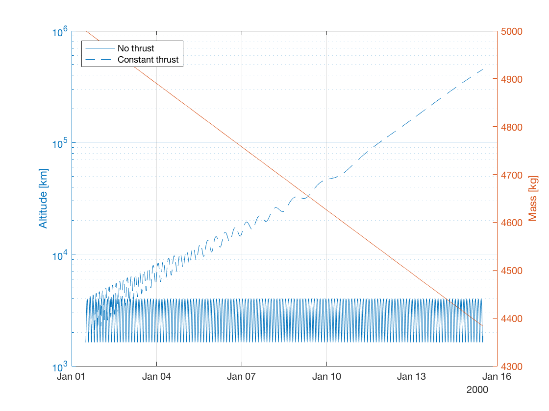
Now we can use the retrieved results to compare the altitudes of the vehicle for the case in which thrust is used and the case in which it is not. We compute the altitude using the function altitude of the package compute, which takes as arguments a matrix of Cartesian states and the body from which to retrieve the average radius. For the case in which thrust is on, we also plot the evolution of the vehicle’s mass:

figure;
grid on;

yyaxis left;
altitudesOff = compute.altitude(statesOff,Earth);
semilogy(convert.epochToDate(epochsOff),altitudesOff/1e3);
ylabel('Altitude [km]');
hold on;

altitudesOn = compute.altitude(statesOn,Earth);
semilogy(convert.epochToDate(epochsOn),altitudesOn/1e3);
legend('No thrust','Constant thrust','Location','NorthWest');
hold off;

yyaxis right;
plot(convert.epochToDate(epochsOn),masses);
ylabel('Mass [kg]');