Multiple propagations

This tutorial describes how to run multiple propagations sharing a set of settings for which just a few parameters are changed in every case using the MATLAB Interface. The code for this example can be found at:

tudatBundle/matlabInterface/Examples/Seamless/multiplePropagations.m

The first step is to include the source code of the MATLAB Interface into MATLAB’s path in the current session so that all the classes needed to set up the simulation can be accessed. This is done by writing:

tudat.load();

Now, we create a Simulation object specifying the initial epoch by providing it as input argument (i.e. 0 seconds since J2000):

simulation = Simulation(0);
simulation.spice.preloadEphemeris = false;

We do not specify a final epoch because there is no time termination condition. Later we will define a termination condition based on the periapsis altitude of the propagated body. Since the propagation period is not known (we know the initial epoch but not the final epoch), the ephemeris of the celestial bodies cannot be preloaded from Spice, so we set simulation.spice.preloadEphemeris to false.

Next, we create the bodies. In this case, the only non-celestial body is named satellite:

satellite = Body('satellite');
satellite.initialState.apoapsisAltitude = 300e3;
satellite.initialState.periapsisAltitude = 200e3;
satellite.initialState.inclination = deg2rad(60);
satellite.initialState.trueAnomaly = deg2rad(45);
satellite.dragCoefficient = 2.5;
satellite.radiationPressureCoefficient = 1.2;
satellite.radiationPressure.Sun.occultingBodies = {Earth};

Now, we add the bodies to the simulation by calling the method addBodies of the simulation object. There exist predefined objects for celestial bodies (namely the Sun, the Moon and the eight planets), so these objects can be added directly without the need to specify their properties:

simulation.addBodies(Earth,Sun,Moon,Mars,Venus,satellite);

Now we need to specify the accelerations acting on satellite:

accelerationsOnSatellite.Earth = {SphericalHarmonicGravity(5,5), AerodynamicAcceleration()};
accelerationsOnSatellite.Sun = {PointMassGravity(), RadiationPressureAcceleration()};
accelerationsOnSatellite.Moon = {PointMassGravity()};
accelerationsOnSatellite.Mars = {PointMassGravity()};
accelerationsOnSatellite.Venus = {PointMassGravity()};

Then, we create the settings for the propagation. We are going to propagate the translational state of the body satellite about Earth. Thus, we use a TranslationalPropagator:

propagator = TranslationalPropagator();
propagator.bodiesToPropagate = {satellite};
propagator.centralBodies = {Earth};
propagator.accelerations.satellite = accelerationsOnSatellite;
simulation.propagators = {propagator};

The next step is to add a termination condition:

simulation.termination = Variable('satellite.periapsisAltitude-Earth') < 105e3;

The propagation will terminate when the perigee altitude gets below 105 km.

Finally, we define the integrator settings, in this case we use a variable step-size Runge-Kutta Fehlberg 7(8) integrator:

integrator = VariableStepSizeIntegrator(RungeKuttaCoefficientSets.rungeKuttaFehlberg78);
integrator.initialStepSize = 60;
integrator.minimumStepSize = 5;
integrator.maximumStepSize = 1e4;
integrator.errorTolerance = 1e-11;
integrator.saveFrequency = 5;
simulation.integrator = integrator;

All the settings needed to run the simulation have been defined, except for the mass and reference area of satellite. In this example, we are going to run the simulation several times for different masses and reference areas, saving the results of each case in a cell array called results:

masses = 200:100:800;
referenceAreas = 8:-1:2;
results = cell(size(masses));
for i = 1:length(masses)
    fprintf('Running case %i of %i...\n',i,length(masses));
    satellite.mass = masses(i);
    satellite.referenceArea = referenceAreas(i);
    simulation.run();
    results{i} = simulation.results.numericalSolution;
end

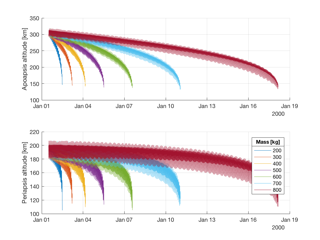
Finally, we can use the saved results to plot the apoapsis and periapsis for each satellite:

figure;
plot.apoapsisPeriapsisAltitudesHistory(results,'CentralBody',Earth);
l = legend(sprintfc('%g',masses));
l.Title.String = 'Mass [kg]';

Note the use of the function apoapsisPeriapsisAltitudesHistory from the plot package. This function takes as first argument a results object, which can be a cell array of results matrices (with epochs in the fist column and Cartesian states in the columns 2 to 7) or a single results matrix. Additional options for plotting can be provided as a set of key-value pairs. The only mandatory argument is the CentralBody, whose average radius is used to compute altitudes. Other optional arguments are TimeUnits, Title, Legends and LineStyle.

This function, as well as the plot.keplerianComponentsHistory function, also accept providing the data to be plotted in other formats. For instance (the first two lines are equivalent):

% results = nx7
plot.apoapsisPeriapsisAltitudesHistory(results,'CentralBody',Earth);
plot.apoapsisPeriapsisAltitudesHistory('CartesianStatesHistory',results,'CentralBody',Earth);
plot.apoapsisPeriapsisAltitudesHistory('KeplerianStatesHistory',results,'CentralBody',Earth);

% epochs = nx1, cartesian = nx6, keplerian = nx6
plot.apoapsisPeriapsisAltitudesHistory('Epochs',epochs,'CartesianStates',cartesian,'CentralBody',Earth);
plot.apoapsisPeriapsisAltitudesHistory('Epochs',epochs,'KeplerianStates',keplerian,'CentralBody',Earth);